H7122-AUTONOMOUS VEHICLES

Question 1:

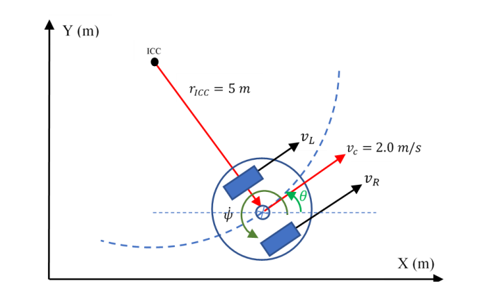
A two-wheel robot with track (i.e., distance between wheels) of 𝑑 = 0.3 𝑚 travels along a circle of radius of 4𝑚, as in Figure Q1-1, with the constant longitudinal speed of 2.0 𝑚/𝑠. 𝐼𝐶𝐶 is the instantaneous centre of curvature. 𝑋 and 𝑌 are ground-fixed axis.

a) Calculate the following variables:

• Longitudinal speeds of the left and right wheels (i.e., 𝑣𝐿 and 𝑣𝑅);

• Yaw rate 𝜓̇;

• Lateral acceleration of each wheel if the distance between the wheels is 20 cm. [8 marks]

b) Calculate the position of the robot after three seconds of travelling. [8 marks]

c) Having autonomous cars on the roads presents benefits and challenges. Name and explain two of the main benefits and three of the main challenges. [4 marks]

Question 2:

a) In Figure Q2-1, if the initial value of the projection of the longitudinal velocity 𝑣𝑐 on the 𝑋 axis (i.e., 𝑉𝑋(0)) is 1 𝑚/𝑠, plot the variation of the projections of 𝑣𝑐 on both the 𝑋 and 𝑌 axis (i.e., 𝑉𝑋 and 𝑉𝑌) along one full rotation of the robot.

b) Explain Bayes’ rule of the probability theory. Discuss the importance of the probability theory and Bayes’ rule to mapping? Using the Bayes’ rule, answer the following question:

You have installed a sensor on your robot that measures the 1-D distance 𝐿 from a reflector with a constant accuracy of ±2 m.

You have fixed the reflector at an accurate distance of 100 m from your reference point (i.e., 𝑓𝐿(100) = 1).

You want to use the sensor to estimate the location of your robot from the readings of the distance of your robot from the reflector (i.e., Pr (𝑥|𝐿)). First, you locate your robot at the positions of {−2, −1,0,1,2} m where you measure several times the distance 𝐿 from the reflector. The distributions of the measurements (i.e., 𝑓𝑋(𝐿|𝑥)) are normal with the mean of respectively {102,101,100,99,98} m and the variance of 1 m.

You locate the robot randomly with uniform distribution at 𝑥𝜖[−2,2] (i.e., 𝑓𝑋(𝑥) = 1/4 ) and measure the distance L from the reflector using your sensor.

If your sensor measures 𝐿 = 100 m, calculate the probability that your robot locates at −1 ≤ 𝑥 ≤ 1 (i.e., Pr (−1 ≤ 𝑥 ≤ 1|𝐿 = 100)). The required values of the normal distribution are as follows:

𝑓𝐿 (100|𝑥 = 0) = 𝒩(100; 𝜇 = 100, 𝜎 = 1) = 0.5;

𝑓𝐿 (100|𝑥 = 1) = 𝑓𝐿 (100|𝑥 = −1) = 𝒩(100; 𝜇 = 99, 𝜎 = 1) = 0.32;

𝑓𝐿 (100|𝑥 = 2) = 𝑓𝐿 (100|𝑥 = −2) = 𝒩(100; 𝜇 = 98, 𝜎 = 1) = 0.074;

c) What is the main problem with the odometrical localisation? Particle filtering (PF) is a technique to solve the simultaneous localisation and mapping (SLAM) problem and is explained in Figure Q2-3. Fill the gaps with the required words to make the sentences meaningful.

Question 3:

We have a Microsoft Kinect camera installed on a Quanser QBot 2 robot. The camera generates both the vision of the environment and distance and orientation of the obstacles as separate vision and depth images.

The depth information, including distance and orientation of the obstacle, is transferred to the processing units as a 2D grey-scale image frame of the size of 480 × 640 pixels (i.e., 480 rows each with 640 pixels).

a) Datasheet of Kinect says that its horizontal field of view (FOV) is 57°. What is the meaning of FOV and how it is related to the motion of the robot for mapping? Figure Q3-1 illustrates the way that Kinect stores the location and orientation information of obstacles within the depth image. If the value of 𝑑 = 6.1m in Figure Q3-1 is stored in the 550th pixel, calculate the distance and orientation of the obstacle 𝑃 (i.e., 𝐿 and 𝛼).

b) According to the formal definition, a transformation (also known as a function) 𝑦𝑖(𝑡) = 𝑇(𝑥𝑖(𝑡)) is linear if and only if:

𝑇(𝑎𝑥1(𝑡) + 𝑏𝑥2(𝑡)) = 𝑎𝑇(𝑥1(𝑡)) + 𝑏𝑇(𝑥2(𝑡)) = 𝑎𝑦1(𝑡) + 𝑏𝑦2(𝑡)

and is time-invariant if and only if for ∀𝜏 ≥ 0:

𝑇(𝑥(𝑡 − 𝜏)) = 𝑦(𝑡 − 𝜏)

Using this definition, evaluate if the following functions are linear or not

c) With providing a mathematical equation and a pseudo code explain the convolution operator between two functions 𝑓(𝑥) and 𝑔(𝑥) and the way it can be implemented as a software programme. Why convolution operator is important for the image processing algorithms? [8 marks]

Question 4:

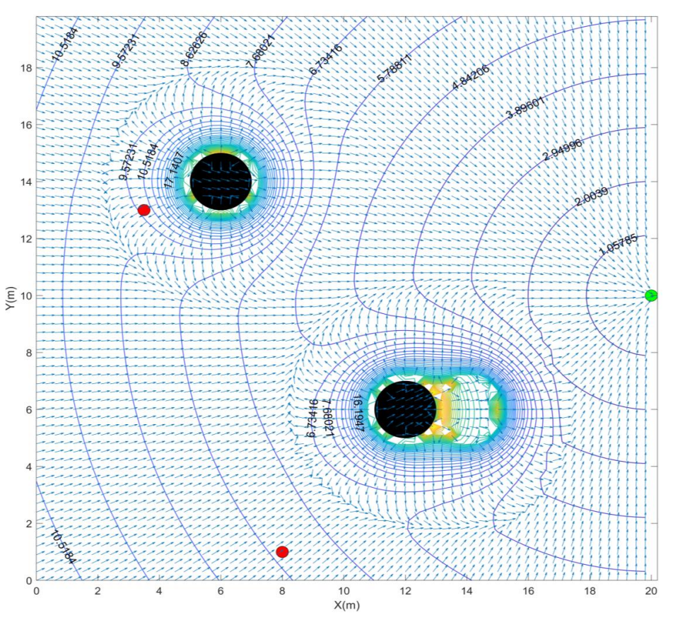
a) Using Figure Q4-1, explain the potential field algorithm for obstacle avoidance. Having the potential fields of Figure Q4-1, how does one calculate the required force to be applied to the robot at each point (𝑥, 𝑦)?

Figure Q4-2 illustrates the resulting potential fields and required force to be applied to the robot at each point (𝑥, 𝑦) to avoid obstacles. Answer the following questions:

• What do the contours show and what do the numbers on them mean?

• What do the blue vectors show at each point of the map?

• What are the black circles in the middle and the green one on the right side of the image? [6 marks]

b) In Figure Q4-2, if a robot is initially located at either of the red circles, suggest the paths that the robot will follow towards its destination. Hint: You need to redraw Figure Q4-2 on your answer sheet as an XY diagram with the obstacles and the initial and destination points and then draw the suggested paths.

Explain the rationale behind your suggested paths.

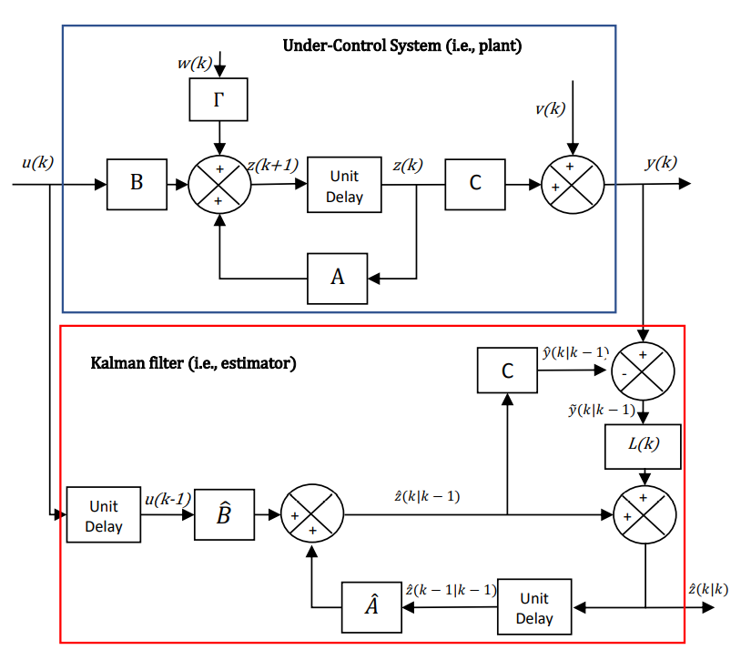
c) Figure Q4-3 shows a Kalman Filter (KF) that estimates the internal state 𝑧(𝑘) of a linear system from a noisy measurement of the system output 𝑦(𝑘). The estimated state is shown as 𝑧̂(𝑘|𝑘) while the system is governed by the following equations:

𝑧(𝑘 + 1) = 𝐴𝑧(𝑘) + 𝐵𝑢(𝑘) + Γ𝑤(𝑘) 𝑦(𝑘) = 𝐶𝑧(𝑘) + 𝑣(𝑘)

As seen, unlike matrices 𝐴 and 𝐵 of the system which are not fully known and estimated as 𝐴̂ and 𝐵̂ to construct KF, matrix 𝐶 is fully known. Also, it is known that the KF gain 𝐿(𝑘) is calculated using the following equation:

𝐿(𝑘) = 𝑃(𝑘|𝑘 − 1)𝐶^𝑇 (𝐶𝑃(𝑘|𝑘 − 1)𝐶 𝑇 + 𝑅𝑣) ^−1

where 𝑃 is the estimated error which is calculated separately and 𝑅𝑣 is the known covariance of the disturbance 𝑣.

Using Figure Q4-3 and the above-mentioned equations, explain the operation of KF. Also, explain the reasons that matrix 𝐶 of a system is fully known and the importance of this phenomenon in KF.